Detecting and classifying signals or correlations present in time series data is a common and important machine learning task. Example applications include, but are not limited to, underwater acoustics (hydrophone data), medical telemetry (EEG, ECG), and system monitoring or predictive maintenance (vibration, temperature, other sensors or metrics).
Sharpe Engineering has developed and created multiple implementations of a signal processing pipeline that has been effective at operating on a wide range of time series data to detect and discriminate targets, biomarkers, and other patterns. Various implementations leveraged of state-of-the-art processing approaches such as Machine Learning, High Performance Stream Processing, and NoSQL data stores and have demonstrated unique capabilities such as the zero-day detection, high levels of discrimination and selectivity, no requirement for labeled training data, and the ability to operate in real-time on large volumes of data.
Pipeline Implementation
The signal processing pipeline outlined below can be easily adapted to a very broad range of types of time series data. While there are certainly opportunities for fine tuning the implementation for a particular use case, some of them such as hyperparameter tuning, can be automated, and others such as the specification of the transformation algorithm(s) can easily be configured using the workflow automation tooling. The general-purpose nature of the approach means that efficacy metrics obtained for one type of signal data will be representative of what could be obtained for many other types.
At a high level, the steps included in the signal processing pipeline listed below combine common processing operations with somewhat more unique fingerprint generation and dimensional reduction capabilities.
Data acquisition (feeding sensor data into the system)
Data cleansing and preparation (filtering out of range values, normalizing range, etc.)
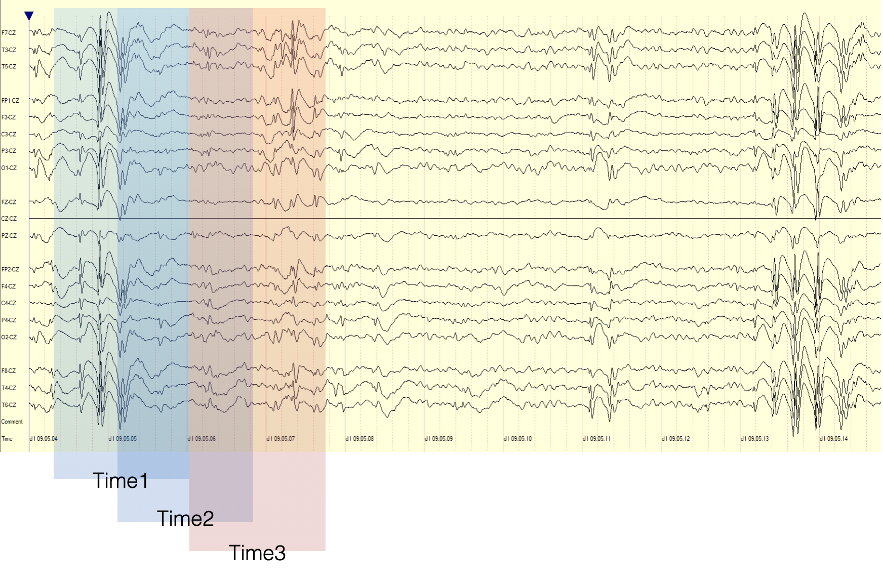
Windowing (grouping portions of the infinite time series data stream into overlapping discretely computable “chunks” as illustrated below)
Transformation (computing a representative “fingerprint” for each window of data. For example, compute the Discrete Fourier, Cosine, or Power Cepstrum and format the respective coefficients into a sequence of bits.
Dimensional reduction (map the high dimensional data produced by the Transformation step down to 2 or 3 dimensions
Classify the resulting low dimensional data. A simple version might consist of bounded areas, but many more options could be used, some of them with quantum support.
Overlapping Sliding Windows

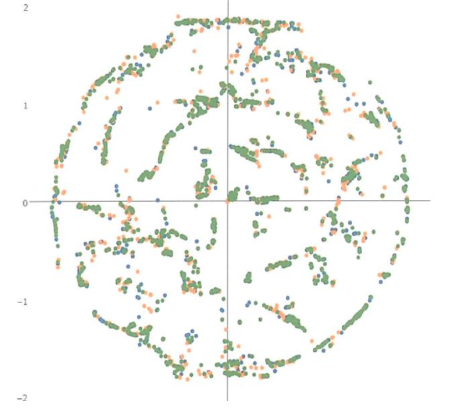
The illustration below Illustrates an example of how the combination of fingerprint generation and dimensional reduction allow the various signals map to locations in lower dimensional space. In this case 3 dimensions. It shows how similar signals tend to be located near each other while also indicating they are different. Two identical signals would map to the same point. This unsupervised machine learning approach simultaneously captures similarities while providing high levels of discrimination. The various distinct locations in the lower dimensional space represent different types of signals. New signal types which have not been previously observed will still be processed by the system but map to locations separate from the other points and therefor be easily noticed.
Relationship between reduced dimensional clusters and the signals they represent

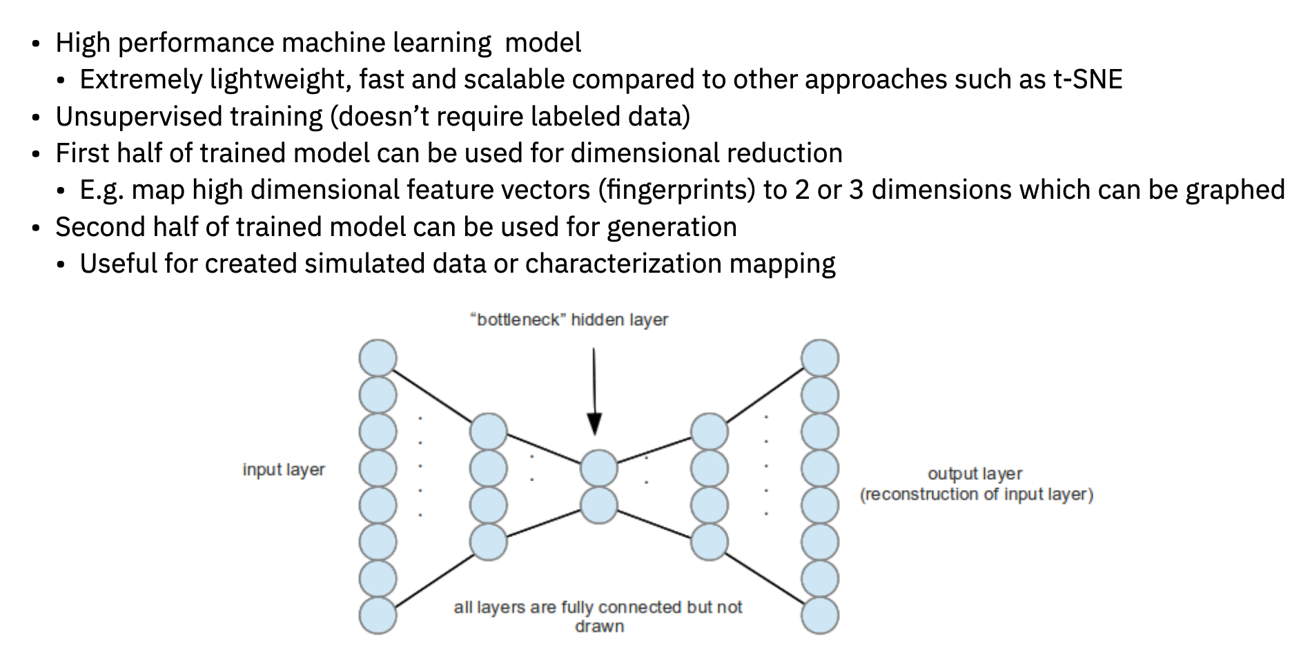
The details of the implementation of the dimensional reduction step are especially important. Previous experience by Sharpe Engineering has shown that using autoencoders for this operation is both effective and highly scalable.
In the illustrated example below of a simple autoencoder, an 8-dimensional input layer is mapped into the 2 dimensions in the “bottleneck” layer. The subsequent layers then map those 2 dimensions back into an 8-dimensional output. This topology allows unsupervised network training since the error is computed by comparing the input data with the generated output. This unsupervised approach means no labelled data is required.
Autoencoder network architecture.

Other algorithms such as t-Distributed Stochastic Neighbor Embedding (t-SNE) can be effective on small amounts of data (see below) and in some situations can scale to large data sets by utilizing data approximation techniques. However, when the data is both large and fast, as is often the case with signal types such as acoustic data, performing the dimensional reduction in real-time requires a different approach.
Example 2d output of using t-SNE Dimensional Reduction on Underwater Acoustic Data

With very minor customization the described pipeline cand be effectively applied to applications as diverse as healthcare telemetry and underwater acoustic data. It’s zero-day capability to detect targets not previously observed or for which there is little available data is an additional benefit as is the removal of the requirement for large amounts of labeled training data.